Next-Word Prediction from Scratch
Building and training a multi-layer perceptron for next-word prediction on a 250-word vocabulary using only NumPy
🎯 Motivation
This project tackles the challenge of next-word prediction in short text sequences using a multi-layer perceptron (MLP) built entirely from scratch using NumPy—no deep learning libraries like TensorFlow or PyTorch. While modern models often depend on large-scale transformer architectures, this work highlights the learning dynamics and architectural challenges of a minimalistic MLP trained on a constrained vocabulary.
The goal was to predict the most likely 4th word given a sequence of 3 input words. With a controlled 250-word vocabulary and fixed-length sequences, the project focuses on foundational principles: embedding representations, forward/backward propagation, and gradient-based optimization.
📎 Links
🧠 Network Architecture
The model predicts the next word by processing three input words in sequence:
- Embedding Layer: Each word index is converted to a one-hot vector and mapped to a 16-dimensional embedding (via matrix multiplication with a learned
W1). - Hidden Layer: The three embeddings are concatenated into a 48-dimensional vector and passed to a hidden layer with 128 units and sigmoid activation.
- Output Layer: A softmax layer predicts a 250-dimensional output representing the probability distribution over the vocabulary.
This model predicts the next word in a sequence using a simple multi-layer perceptron (MLP) with an embedding layer. All computations — forward and backward — are implemented from scratch using NumPy, following precise matrix calculus.
🔢 Mathematical Formulation
Before diving into implementation, we derive the complete forward and backward propagation steps from first principles. This ensures correct dimensionality, transparency in training dynamics, and a solid foundation for debugging and experimentation.
🧮 Forward Propagation
Step 1 – Word Embeddings
Each of the 3 input words is represented as a one-hot vector \(\mathbf{x}_i \in \mathbb{R}^{250}\). These are projected into a continuous space using a shared embedding matrix \(\mathbf{W}_1 \in \mathbb{R}^{250 \times 16}\):
Step 2 – Concatenation
We stack the three embeddings into a single input vector:
Step 3 – Hidden Layer (Linear + Sigmoid)
Using weights \(\mathbf{W}_2 \in \mathbb{R}^{48 \times 128}\) and biases \(\mathbf{b}_1 \in \mathbb{R}^{128}\):
\(\mathbf{z}_1 = \mathbf{h}_0 \cdot \mathbf{W}_2 + \mathbf{b}_1 \in \mathbb{R}^{128}\) \(\mathbf{h}_1 = \sigma(\mathbf{z}_1) = \frac{1}{1 + e^{-\mathbf{z}_1}} \in \mathbb{R}^{128}\)
Step 4 – Output Layer (Linear + Softmax)
Project to vocabulary size using \(\mathbf{W}_3 \in \mathbb{R}^{128 \times 250}\), \(\mathbf{b}_2 \in \mathbb{R}^{250}\):
\(\mathbf{z}_2 = \mathbf{h}_1 \cdot \mathbf{W}_3 + \mathbf{b}_2 \in \mathbb{R}^{250}\) \(\hat{\mathbf{y}} = \text{softmax}(\mathbf{z}_2) = \frac{e^{\mathbf{z}_2}}{\sum_{j=1}^{250} e^{\mathbf{z}_2^{(j)}}} \in \mathbb{R}^{250}\)
🧾 Loss Function: Cross-Entropy
We minimize the cross-entropy between the one-hot encoded target \(\mathbf{y} \in \mathbb{R}^{250}\) and predicted distribution \(\hat{\mathbf{y}}\):
\[\mathcal{L} = -\sum_{j=1}^{250} y_j \log(\hat{y}_j)\]For mini-batch of size ( n ):
\[\mathcal{L} = -\frac{1}{n} \sum_{i=1}^{n} \sum_{j=1}^{250} y_{ij} \log(\hat{y}_{ij})\]🔁 Backward Propagation
Step 1 – Error at Output Layer
\[\delta_3 = \hat{\mathbf{y}} - \mathbf{y} \in \mathbb{R}^{250}\]Step 2 – Gradients for Output Layer
\[\nabla \mathbf{W}_3 = \mathbf{h}_1^\top \cdot \delta_3 \quad \nabla \mathbf{b}_2 = \delta_3\]Step 3 – Backprop Through Sigmoid
\[\delta_2 = (\delta_3 \cdot \mathbf{W}_3^\top) \odot \mathbf{h}_1 \odot (1 - \mathbf{h}_1)\]Step 4 – Gradients for Hidden Layer
\[\nabla \mathbf{W}_2 = \mathbf{h}_0^\top \cdot \delta_2 \quad \nabla \mathbf{b}_1 = \delta_2\]Step 5 – Backprop to Embedding Layer
Let:
Split into:
\[[\delta_{e_1}, \delta_{e_2}, \delta_{e_3}] \in \mathbb{R}^{16}\]Update embedding matrix:
\[\nabla \mathbf{W}_1 += \delta_{e_i} \cdot \mathbf{x}_i^\top \quad \text{for } i = 1, 2, 3\]This explicit breakdown aligns with the core training algorithm implemented in NumPy and mirrors full symbolic derivation in standard deep learning texts.
⚗️ Experimentation & Insights
A wide range of experiments were conducted to understand what impacts model learning the most:
| Category | Variants Explored |
|---|---|
| Initialization | Zero, Random, Xavier (final) |
| Learning Rate | 0.1, 0.01 (final), 0.001 |
| Batch Size | 10, 50, 100 (final), 200, 500 |
| Epochs | 10, 20 (final), 50 |
| Weight Updates | Manual SGD via backward propagation |
| Evaluation Strategy | Per-epoch validation + test accuracy |
Findings:
- Zero initialization failed due to symmetry.
- Xavier initialization worked best for sigmoid.
- Batch size impact was minimal only under optimal learning rates.
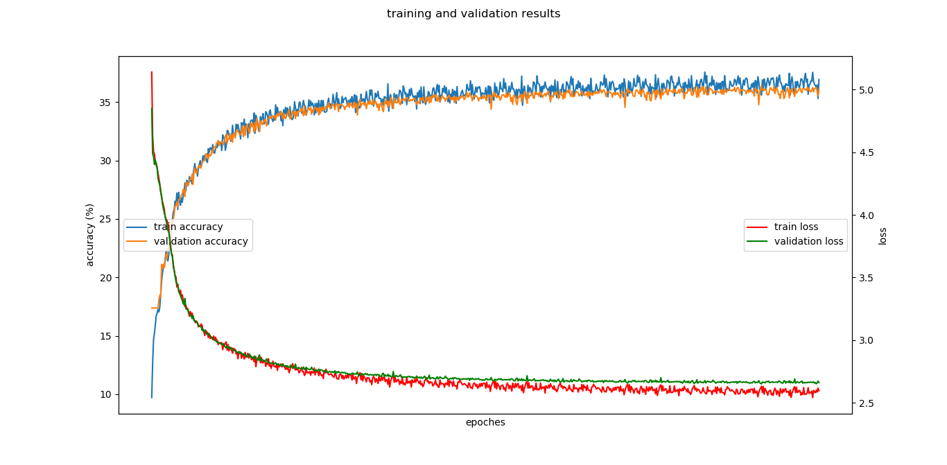
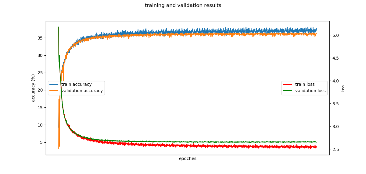
- Final performance reached ~36% accuracy — competitive given limited expressiveness and no pretrained embeddings.
📉 Performance Visualization
To monitor convergence, training and validation accuracy/loss were recorded per epoch. Results revealed that convergence stabilized after ~20 epochs, motivating early stopping.


🧬 Word Embedding Visualization
To inspect learned word semantics, the 16-dimensional embedding vectors were reduced to 2D using t-SNE, producing several semantically or syntactically coherent clusters:
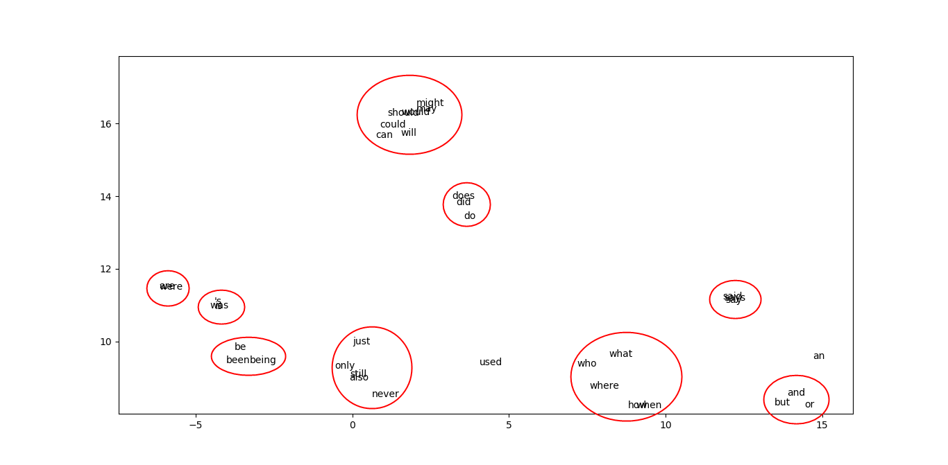
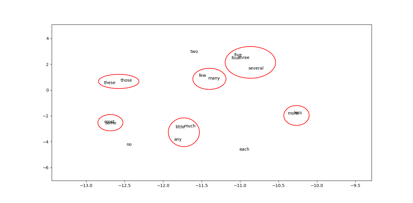
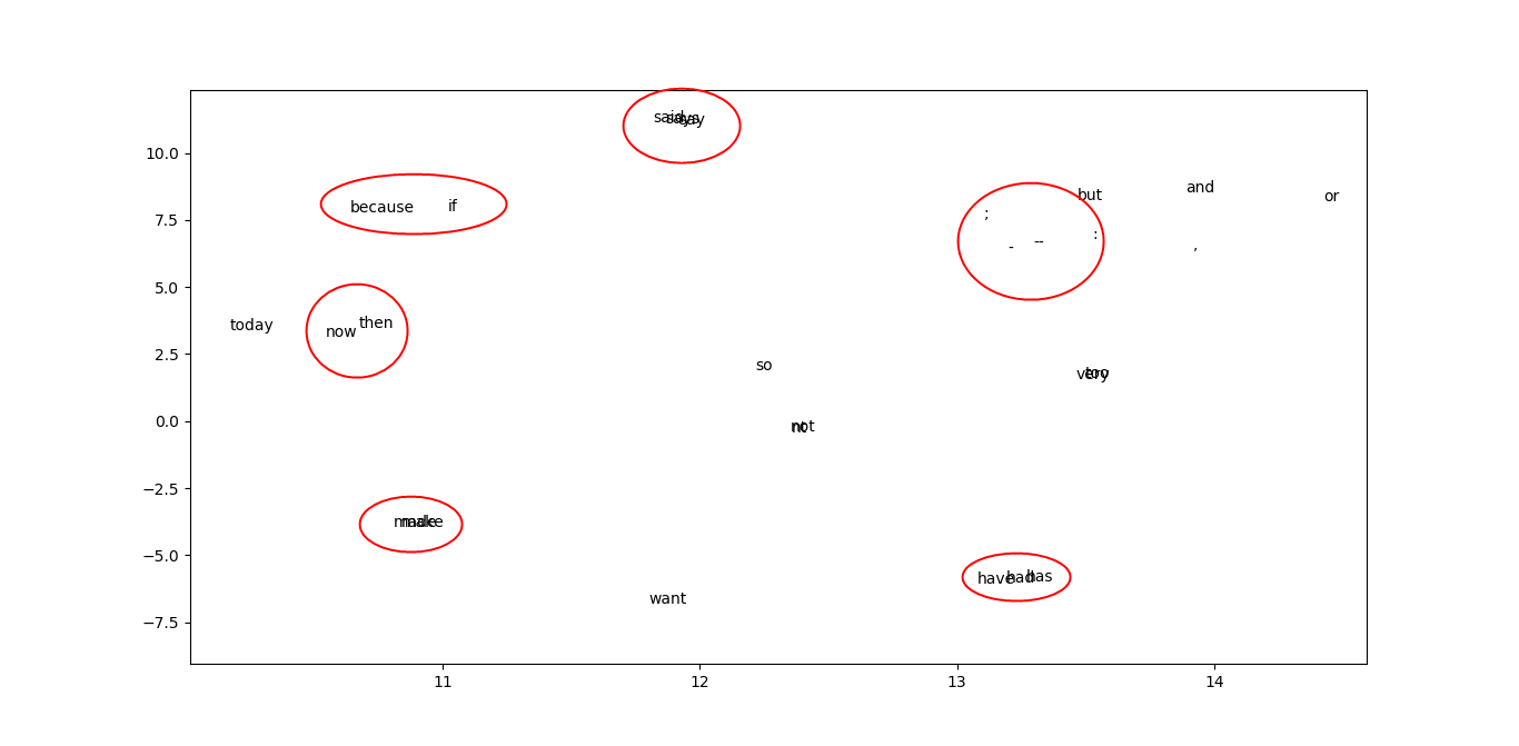
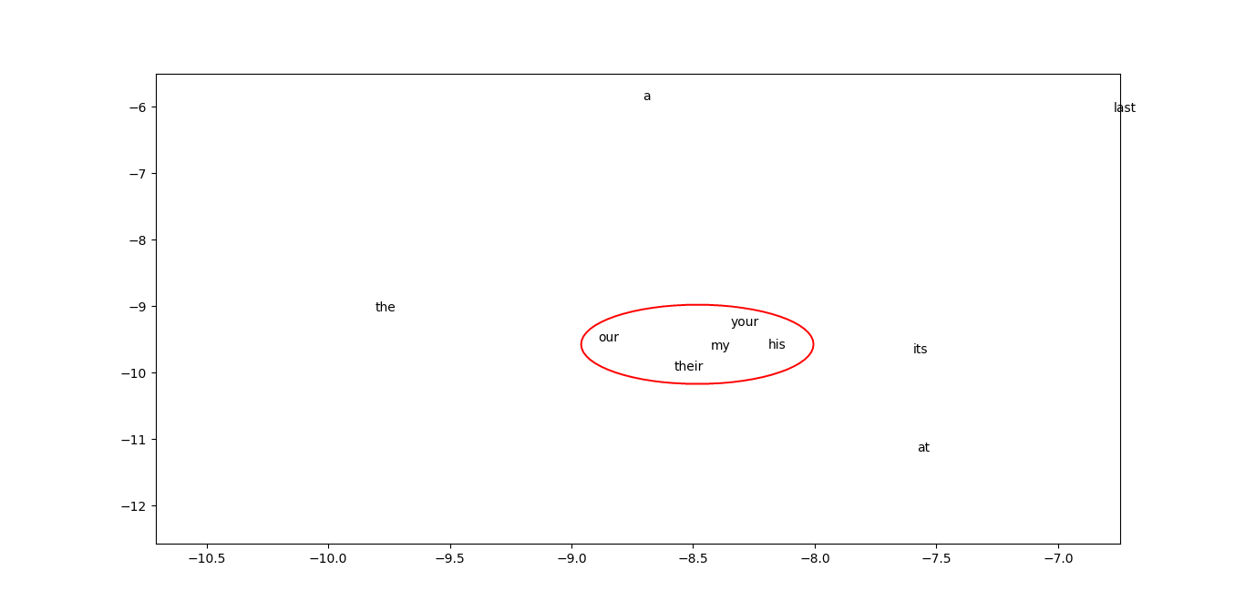
Examples include:
- Modals: can, could, might, should
- Pronouns: my, your, their, his
- Temporal: now, then, today
- Conjunctions: and, but, or
📌 Sample Predictions
The trained model could generate grammatically and semantically valid next-word predictions:
| Input Sequence | Predicted Word |
|---|---|
| city of new | york |
| life in the | world |
| he is the | best |
These results reflect learned sequential patterns despite architectural simplicity.
⚙️ Technical Stack
- Language: Python (NumPy only)
- Network: 1 hidden layer MLP with embeddings
- Optimization: Custom backward propagation & SGD
- Evaluation: Accuracy, Loss, Manual t-SNE, Prediction sampling