Expectation-Maximization for GMM from Scratch
Step-by-step implementation of the expectation-maximization (EM) algorithm for Gaussian mixture models (GMMs) from scratch
🎯 Motivation
This project demonstrates how the Expectation-Maximization (EM) algorithm can be used to fit a Gaussian Mixture Model (GMM) to unlabeled data. Unlike K-means, GMM with EM models data as a combination of probabilistic clusters with soft assignments, providing more flexible and realistic representations of real-world data.
The implementation was built from scratch in Python, with custom logic for the E-step and M-step. Visualizations of how cluster assignments evolve over iterations provide valuable intuition on the convergence behavior and sensitivity to initialization.
📎 Links
🧠 Algorithm Summary
We aim to fit the data with \(K = 3\) Gaussian components. The EM algorithm proceeds iteratively with the following two steps:
- E-step: Compute soft cluster assignments (responsibilities) for each point using current estimates of means, covariances, and mixture weights.
- M-step: Update the parameters (means, covariances, and weights) by maximizing the expected log-likelihood based on current responsibilities.
Convergence is detected when the increase in log-likelihood falls below a defined threshold (e.g., \(\epsilon = 10^{-4}\)).
📊 Iterative Clustering Process
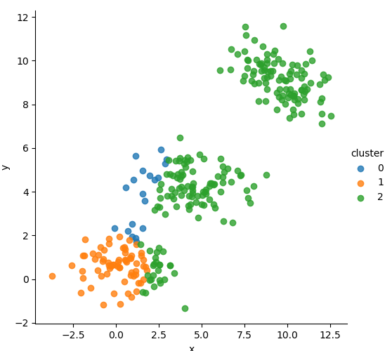
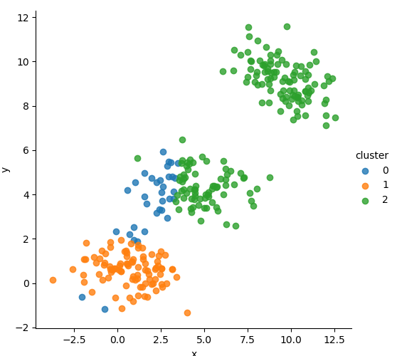
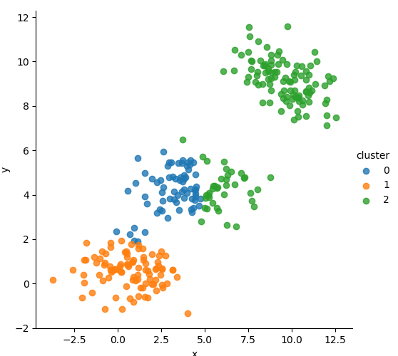
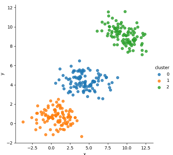
We tracked the cluster assignment evolution visually across several EM steps, revealing how the model gradually finds the optimal Gaussian boundaries.


🧮 Mathematical Formulation
Let \(\mathbf{x}_i \in \mathbb{R}^d\) be the input data point, and let \(\pi_k\), \(\mu_k\), and \(\Sigma_k\) be the weight, mean, and covariance matrix for component \(k\).
Gaussian PDF
The likelihood of point \(\mathbf{x}_i\) under component \(k\) is given by:
\[\mathcal{N}(\mathbf{x}_i \mid \mu_k, \Sigma_k) = \frac{1}{(2\pi)^{d/2} |\Sigma_k|^{1/2}} \exp\left(-\frac{1}{2} (\mathbf{x}_i - \mu_k)^\top \Sigma_k^{-1} (\mathbf{x}_i - \mu_k)\right)\]E-step: Responsibility Calculation
Soft assignment \(\gamma_{ik}\) of point \(i\) to cluster \(k\):
\[\gamma_{ik} = \frac{\pi_k \, \mathcal{N}(\mathbf{x}_i \mid \mu_k, \Sigma_k)}{\sum_{j=1}^K \pi_j \, \mathcal{N}(\mathbf{x}_i \mid \mu_j, \Sigma_j)}\]M-step: Parameter Updates
Weighted sums:
\[N_k = \sum_{i=1}^n \gamma_{ik}\]Updated mean:
\[\mu_k = \frac{1}{N_k} \sum_{i=1}^n \gamma_{ik} \mathbf{x}_i\]Updated covariance:
\[\Sigma_k = \frac{1}{N_k} \sum_{i=1}^n \gamma_{ik} (\mathbf{x}_i - \mu_k)(\mathbf{x}_i - \mu_k)^\top\]Updated mixture weight:
\[\pi_k = \frac{N_k}{n}\]Log-Likelihood
To track convergence:
\[\log p(X) = \sum_{i=1}^n \log \left( \sum_{k=1}^K \pi_k \, \mathcal{N}(\mathbf{x}_i \mid \mu_k, \Sigma_k) \right)\]📈 Sensitivity to Initialization
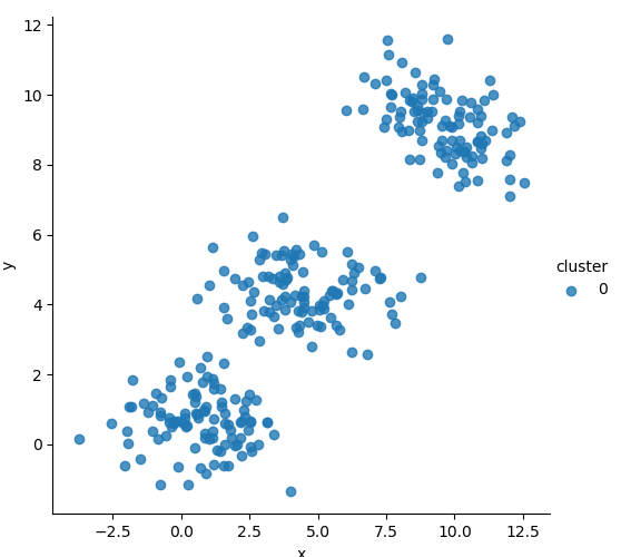
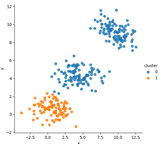
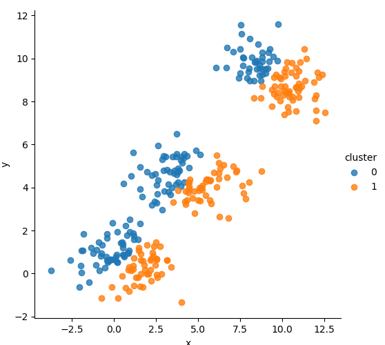
Different random initializations lead to different convergence paths. Below are examples starting from various initial guesses for means:

🧪 Additional Explorations
- Tracked log-likelihood evolution across iterations
- Explored different covariance strategies (diagonal vs. full)
- Compared soft vs. hard assignments (vs. K-means)
- Visualized 2D projections of posterior probabilities
- Confirmed convergence stability and repeatability
⚙️ Technical Stack
- Language: Python (NumPy, Matplotlib, Seaborn)
- Algorithm: Expectation-Maximization for Gaussian Mixture Models
- Visualization: Iterative clustering, posterior surfaces, convergence curves
- Evaluation: Log-likelihood trends, cluster interpretability, sensitivity analysis